
How artificial intelligence improves radio propagation modelling: methods, accuracy trade-offs, training data needs, and a practical deployment workflow.
Propagation Modelling Artificial Intelligence
Radio propagation modelling predicts how a wireless signal weakens and scatters as it travels from a transmitter to a receiver. For decades engineers relied on two families of tools: fast empirical formulas that were cheap but approximate, and physics-based ray tracing that was accurate but slow. Artificial intelligence is now being used as a third option, one that learns the relationship between the environment and the received signal directly from data. This article explains how that works, where it genuinely helps, where it fails, and how to build a workflow you can trust.
Quick Answer: Propagation modelling artificial intelligence uses machine learning models trained on measured or simulated radio data to predict path loss and coverage. Neural networks learn terrain, building, and frequency effects directly from data, delivering ray-tracing-level detail at far lower compute cost, provided the training data represents the target environment.
Table of Contents
- What Propagation Modelling Means in Practice
- Why Traditional Models Hit a Ceiling
- How AI Learns Propagation Behaviour
- Comparison of Propagation Modelling Approaches
- What Training Data You Actually Need
- Where AI Propagation Models Fail
- A Practical Deployment Workflow
- Key Takeaways
- Frequently Asked Questions
What Propagation Modelling Means in Practice
Propagation modelling answers one measurable question: what is the signal strength at a given point, given a transmitter location, frequency, antenna configuration, and environment? The core output is path loss, expressed in decibels, which is the difference between transmitted and received power.
Accuracy is normally judged by root mean square error against measurements. Classical empirical models such as Okumura-Hata and COST 231 commonly show RMSE in the range of roughly 8 to 12 dB in real urban deployments, while calibrated deterministic methods can reach the 4 to 7 dB range. That gap matters commercially, because every additional decibel of prediction error forces engineers to add link margin, and extra margin means more sites, more power, or reduced capacity.
Key Terms Defined
- Path loss: attenuation of signal power between transmitter and receiver, in dB.
- Shadowing: slow variation in signal caused by obstruction from terrain and buildings.
- Small-scale fading: rapid fluctuation from multipath interference over short distances.
- Ray tracing: deterministic simulation that traces reflection, diffraction, and scattering paths.
Why Traditional Models Hit a Ceiling
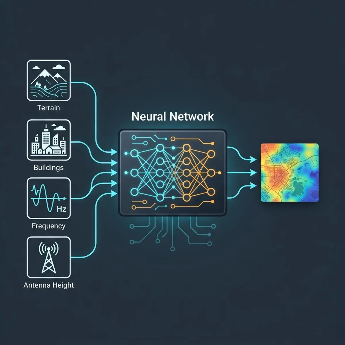
Traditional models struggle because they compress a complex three-dimensional environment into a handful of scalar parameters. An empirical model typically knows distance, frequency, antenna heights, and a broad clutter class such as urban or suburban. It does not know that a specific street canyon runs parallel to the boresight, or that a glass tower sits 40 metres behind the receiver.
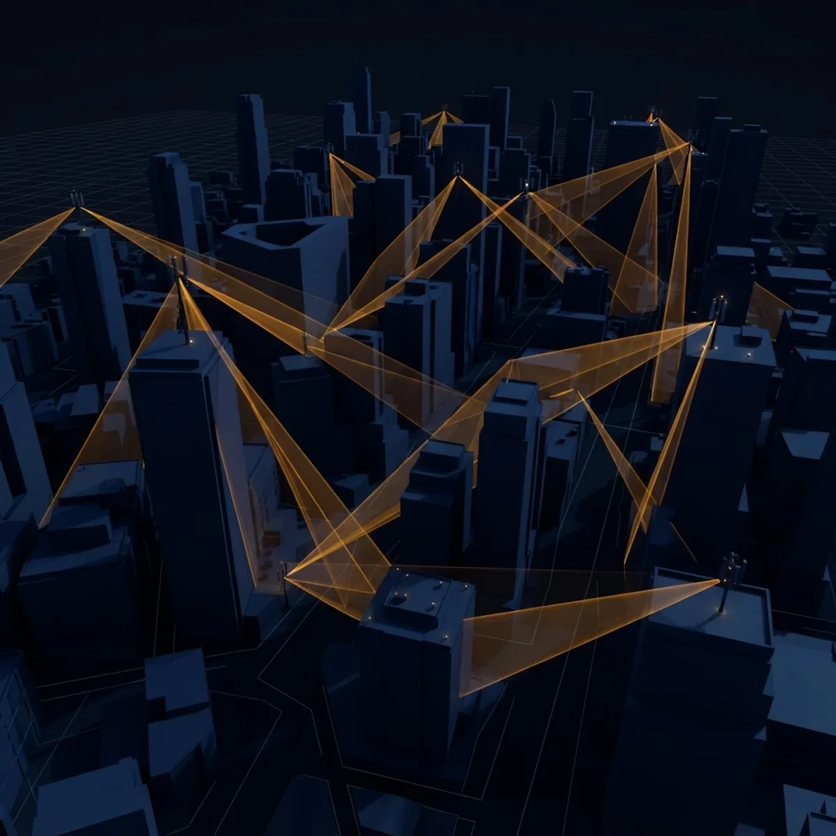
Ray tracing solves that by modelling geometry explicitly, but the computational cost grows quickly with the number of surfaces and the interaction order. A detailed dense-urban ray-tracing run over several square kilometres can take minutes to hours per transmitter on standard hardware. When a planning team needs to evaluate thousands of candidate site configurations, or when a network needs coverage predictions refreshed continuously, that cost becomes the binding constraint rather than accuracy.
This is the practical opening for machine learning. AI does not invent new physics. It approximates an expensive function cheaply, and it can extract patterns from environmental data that hand-built formulas discard.
How AI Learns Propagation Behaviour
AI propagation models treat prediction as a supervised learning problem: given features describing the environment and link geometry, predict received power or path loss. Three architectural families dominate current work.
Tabular Models for Scalar Features
Gradient boosting and random forests work on engineered features such as distance, frequency, effective antenna height, terrain profile statistics, building density, and land-use class. These models train in minutes on modest datasets, are easy to interpret through feature importance, and often beat empirical formulas by a meaningful margin. They are the correct starting point when you have tens of thousands of measurement records but no reliable 3D building data.
Convolutional Networks for Map Inputs
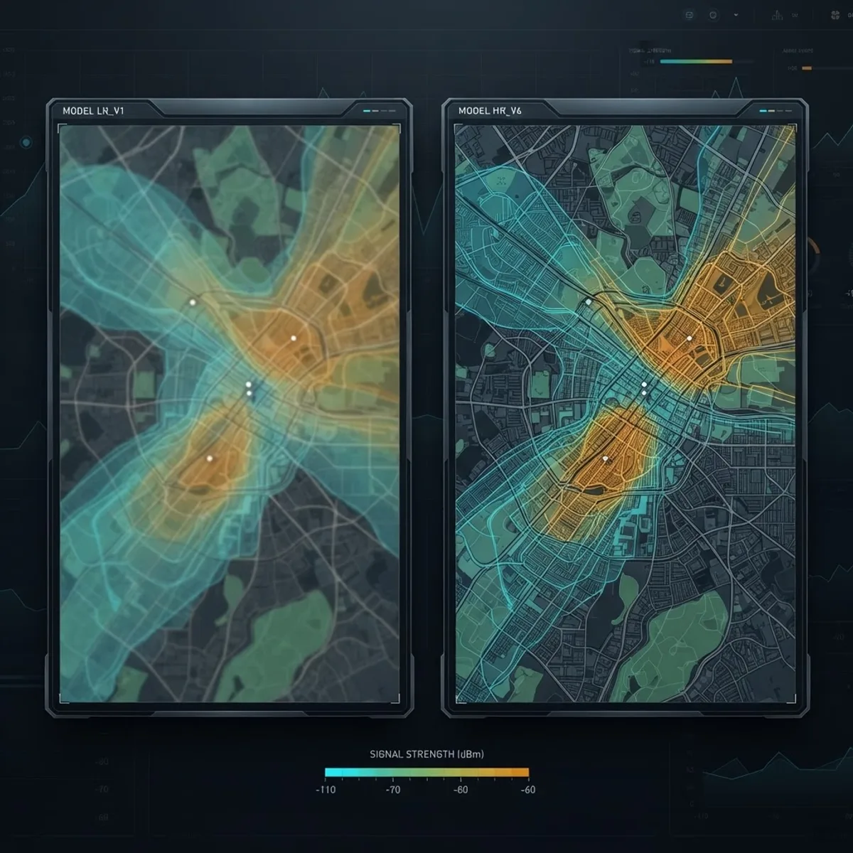
Convolutional neural networks accept the environment as image-like layers: a building height raster, terrain elevation, land cover, and the transmitter position. The network then outputs a full coverage map in a single forward pass. Because a CNN sees spatial structure, it can learn shadowing behind obstacles rather than averaging it away. Published research on learned radio map prediction, including the widely cited RadioUNet work, reports inference in milliseconds per map, several orders of magnitude faster than the ray-tracing simulations used to generate the training labels.
Graph and Physics-Informed Models
Graph neural networks represent scatterers and interaction points as nodes, which suits multipath problems where relationships matter more than pixel grids. Physics-informed approaches go further by constraining the model with known behaviour, for example enforcing free-space loss as a baseline and letting the network predict only the residual correction. Residual learning is one of the most reliable practical tricks available, because the model starts from a physically valid prediction and never produces wildly unphysical output in unfamiliar conditions.

Comparison of Propagation Modelling Approaches
| Approach | Typical accuracy | Compute cost | Data requirement | Best fit |
|---|---|---|---|---|
| Empirical formula | Lowest, wide error spread | Negligible | None | Early feasibility studies |
| Calibrated empirical | Moderate | Very low | Modest measurement set | Regional planning at scale |
| Ray tracing | Highest with good geometry | Very high | Accurate 3D city model | Dense urban and mmWave design |
| Tabular machine learning | Moderate to good | Low | Tens of thousands of samples | Measurement-rich, geometry-poor cases |
| Convolutional network | Good to high | Low at inference, high at training | Large map and label dataset | Fast repeated coverage prediction |
| Hybrid or physics-informed | High and more stable | Moderate | Smaller than pure data models | Production systems needing reliability |
The pattern is consistent: AI shifts cost from inference time to training time. That trade is worthwhile when predictions are requested repeatedly and unprofitable when you need one map once.
What Training Data You Actually Need
Data quality decides outcomes more than architecture choice. A well-tuned gradient boosting model on clean, well-labelled data will usually outperform a sophisticated network trained on noisy or misaligned inputs.
Measurement Data
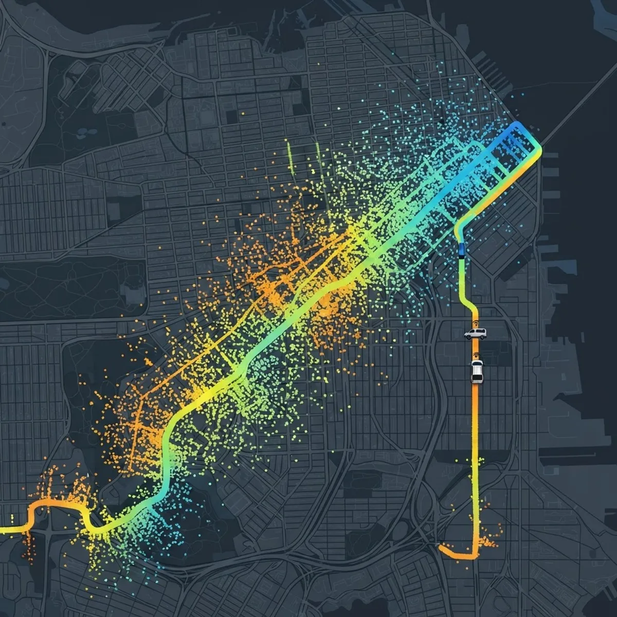
Drive test and crowdsourced measurements provide ground truth but carry known defects. GPS error of 5 to 10 metres in urban canyons can misalign a sample with its true clutter context. Receiver hardware differences introduce systematic offsets. Drive routes also oversample roads and undersample indoor and elevated positions, which biases any model trained naively on them.
Simulated Data
Ray-tracing output offers unlimited, perfectly labelled samples with full spatial coverage, which is why most published learned radio map models train on simulation. The limitation is that the model learns the simulator, including its errors and its assumptions about material properties. The standard mitigation is transfer learning: pre-train on large simulated datasets, then fine-tune on the smaller real measurement set from the target region.
Environmental Layers
Useful inputs include building footprints with heights, digital terrain and surface models, land cover classification, road networks, and vegetation indices. Resolution should match the wavelength scale of interest. Sub-6 GHz planning tolerates 10 to 25 metre rasters, while millimetre wave work generally needs 1 to 5 metre detail because a single missing wall changes the outcome entirely.
Where AI Propagation Models Fail
Being explicit about limitations is what separates a usable model from a demo.
- Generalisation across cities. A model trained on one urban morphology often degrades sharply elsewhere. Always validate on a geographically held-out area rather than a random split, because random splits leak neighbouring samples between train and test.
- Frequency extrapolation. Interpolating between trained frequency bands is reasonable. Extrapolating from 2 GHz training data to 28 GHz is not, because dominant physical mechanisms change.
- No usable uncertainty by default. A point prediction gives planners no confidence information. Quantile regression, ensembles, or Monte Carlo dropout give an error range engineers can convert into link margin.
- Silent data drift. New construction changes the environment while the model does not. Predictions degrade quietly, so monitoring residuals against fresh measurements is mandatory.
- Limited explainability. When a network predicts unexpectedly weak coverage, tracing the cause is harder than in ray tracing, where individual paths are inspectable.
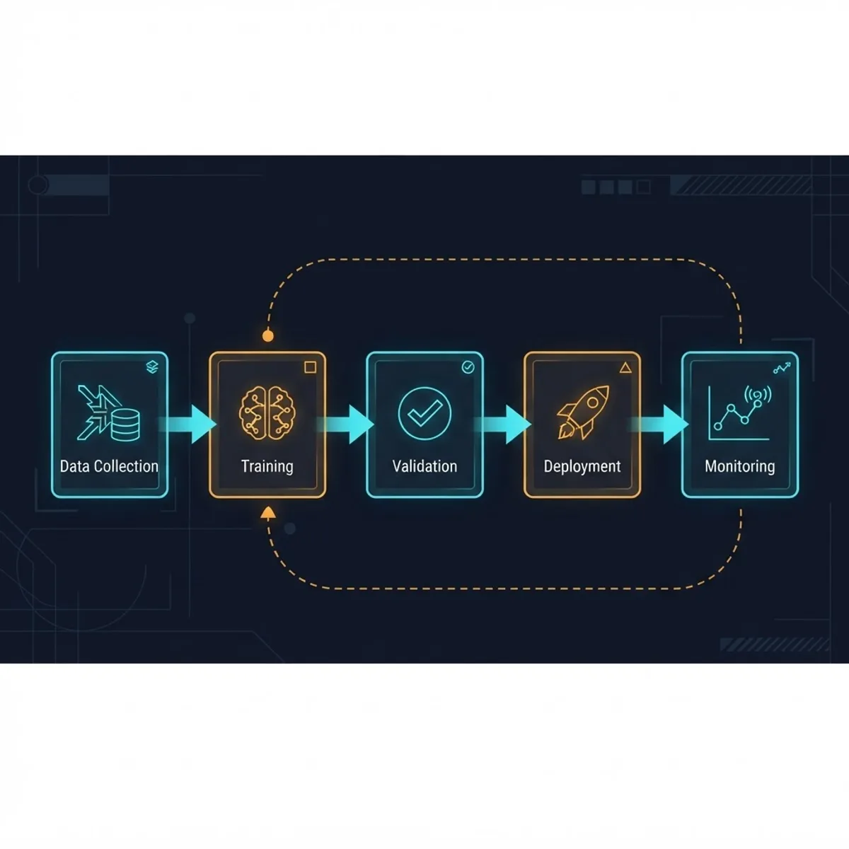
A Practical Deployment Workflow
Follow these steps to move from concept to a maintained production model.
- Define the decision the model supports. Site selection, capacity planning, and interference analysis need different accuracy and resolution. Set a target RMSE before modelling.
- Establish a baseline. Fit a calibrated empirical model first. It is your minimum acceptable performance and takes hours, not weeks.
- Assemble and align data. Snap measurements to environmental rasters, remove GPS-implausible points, and normalise receiver offsets per device type.
- Split by geography. Hold out whole districts for validation and a separate region for final testing.
- Train the simplest sufficient model. Start with gradient boosting on engineered features, then progress to a CNN only if map-level detail is required.
- Predict residuals, not raw path loss. Anchoring the model to a physical baseline improves stability outside training conditions.
- Quantify uncertainty. Output prediction intervals alongside point estimates so planners can size margin rationally.
- Monitor and retrain. Track residual drift quarterly and retrain when error exceeds your defined threshold.
Teams building the surrounding tooling, dashboards, and data pipelines for this kind of system often pair RF specialists with engineers who handle the software layer, and working with a partner such as full stack AI solutions providers can shorten that path. For the model-serving and inference infrastructure itself, custom AI models work is where most of the engineering effort ultimately lands.
Key Takeaways
- Propagation modelling predicts path loss in dB; empirical models commonly show roughly 8 to 12 dB RMSE in urban settings versus 4 to 7 dB for calibrated deterministic methods.
- AI models mainly convert expensive simulation into cheap inference, with learned radio map methods reporting millisecond-scale predictions.
- Convolutional networks suit full coverage maps; gradient boosting suits scalar feature datasets without 3D geometry.
- Residual or physics-informed learning improves stability by anchoring predictions to known physics.
- Validate on geographically held-out areas, never random splits, to measure real generalisation.
- Millimetre wave modelling requires 1 to 5 metre environmental resolution; sub-6 GHz tolerates 10 to 25 metre rasters.
- Uncertainty estimates and drift monitoring are requirements, not optional extras, in production networks.
Frequently Asked Questions (FAQ)
What is propagation modelling in artificial intelligence?
It is the use of machine learning models to predict radio signal path loss and coverage from environmental and link data. Instead of applying fixed formulas, the model learns propagation behaviour from measured or ray-traced examples, then predicts signal strength for new locations in milliseconds.
Is AI more accurate than ray tracing for propagation prediction?
Not inherently. Ray tracing with accurate 3D geometry remains the accuracy reference. AI models trained on ray-tracing output approximate it closely while running far faster. Accuracy depends heavily on training data coverage, so AI typically wins on speed and scale rather than raw precision.
How much data do I need to train a propagation model?
Tabular models can produce useful results with tens of thousands of aligned measurement samples. Convolutional map-based models generally require thousands of simulated coverage maps. A common efficient approach is pre-training on simulated data, then fine-tuning with a few thousand local real measurements.
Can one AI propagation model work for every city?
Rarely without adaptation. Building density, height distribution, and materials differ enough that accuracy drops when a model is applied to unfamiliar morphology. Fine-tuning on local measurements, or including morphology features explicitly during training, substantially improves cross-city transfer performance.
Which machine learning method should I start with?
Start with gradient boosting on engineered features such as distance, frequency, antenna heights, and terrain statistics. It trains quickly, is interpretable, and establishes whether your data supports learning at all. Move to convolutional networks only when you need full spatial coverage maps.